SAM
Introduction
This blogpost deals with a statistical analysis for gene expression microarray experiments, called Significance Analysis of Microarrays (SAM) , that - despite the name - is not restricted for microarray analysis [1] but serves as a blue print for any permutation test.
When performing a microarray of differentially expressed genes, you capture a snapshot of transcriptional activity in different biological states (for example control vs. heat stress) and want to identify differences in those states.
Therefore, all genes in a cell are measured, which leads to an immense amount of data (high throughput method).
Those experiments can be used to identify all differentially expressed genes, not only small subsets contrary to traditional approaches.
Those identifications can lead to the discovery of new functional roles or mechanisms of genes involved in (stress) responses.
The main goal is therefore to identify all differentially expressed genes with a controlled number of false positives.
This approach leads to the following problems handling immense datasets in contrast to traditional analysis:
- The need of computational capacity and
- the control of multiple testing errors
The first one can be overcome easily nowadays, but the multiple testing errors remain a challenge. Hypothesis tests report a p value, that corresponds to the probability of obtaining results at least as extreme as the observed results, assuming that the null hypothesis is correct. In other words: If there is no effect (no mean difference), a p value of 0.05 indicates that in 5 % of the tests a false positive is reported.
Example: You investigate 10.000 genes and perform standard t-tests. With a p value of 5 % (alpha level 0.05), on average 500 tests will be reported as significantly different without being different (false positives).
Traditional statistical tests like t-tests were originally created to perform comparisons between one test only, not 10.000. With an increasing number of performed tests the probability of encountering false positives increases. This effect can be adjusted or minimized by applying correction methods. Correction methods, like Bonferroni, usually account for the number of performed tests, lowering the threshold (BonferroniThreshold) for calling a change significant.

With this lowered threshold it is more likely to miss true differentially expressed genes.
Using the example from above, an alpha level of 0.05 and 10.000 performed tests results in a p value of 0.000005 for genes to be called significant.
This high number of comparisons is not unusual in modern experiments and therefore needs a new approach to overcome the multiple testing error problem.
One approach is the usage of the False-Discovery-Rate FDR instead of p values, for the reason that it is robust to false positives and is widely used in exploratory analysis where the goal is to have mostly true findings and a minimum of false positive findings.
The FDR describes the rate of expected false positives in all significant findings.
Another concern in differential gene expression analysis is failing to identify truly differentially expressed genes, which is why the FDR is used (as many true positives with minimum of false positives). For further information see the q values BlogPost.
A second approach is using q values, which are local FDRs of single genes in this case.
Every gene with a greater significance than the one observed will be called significant, and provides a higher accuracy than conventional t-tests according to the initial publication of SAM [1].
Solution
SAM (Significance Analysis of Microarrays) is a tool developed to overcome this multiple testing problem. It is a statistical method for multiple hypothesis testing and is mainly used for differential gene expression analysis. It is able to compare different biological states with thousands of genes without the loss of true positive findings due to before mentioned correction methods. The first application of SAM was studying the influence of ionizing radiation on the transcriptional response of lymphoblastoid cells in 2001[1]. They found 34 differentially expressed genes, 19 involved in cell cycle regulation and 3 in apoptosis.
The focus is the comparison of different experimental states and to identify changes. To identify changes, it is crucial to know how the data would act if there is no change. But in biological experiments, it is often challenging to define the true null distribution (no change). This leads to a complex problem that needs a tailored solution. SAM accounts for this problem with a combined permutation-bootstrap-method. Bootstrap method here means that a new dataset is created out of the available observed data by random sampling and can be used as a no change reference (synthetic null distribution). The relation of data to their treatment is lost and therefore, each reported positive result is a false positive. To compare different states a statistic is calculated for each observed gene and the expected values from the bootstrap method (synthetic null distribution). More extreme statistics are more likely to be true changes and less likely to occur by chance. With a high statistic, the chances are high to find a real difference between control and treatment.
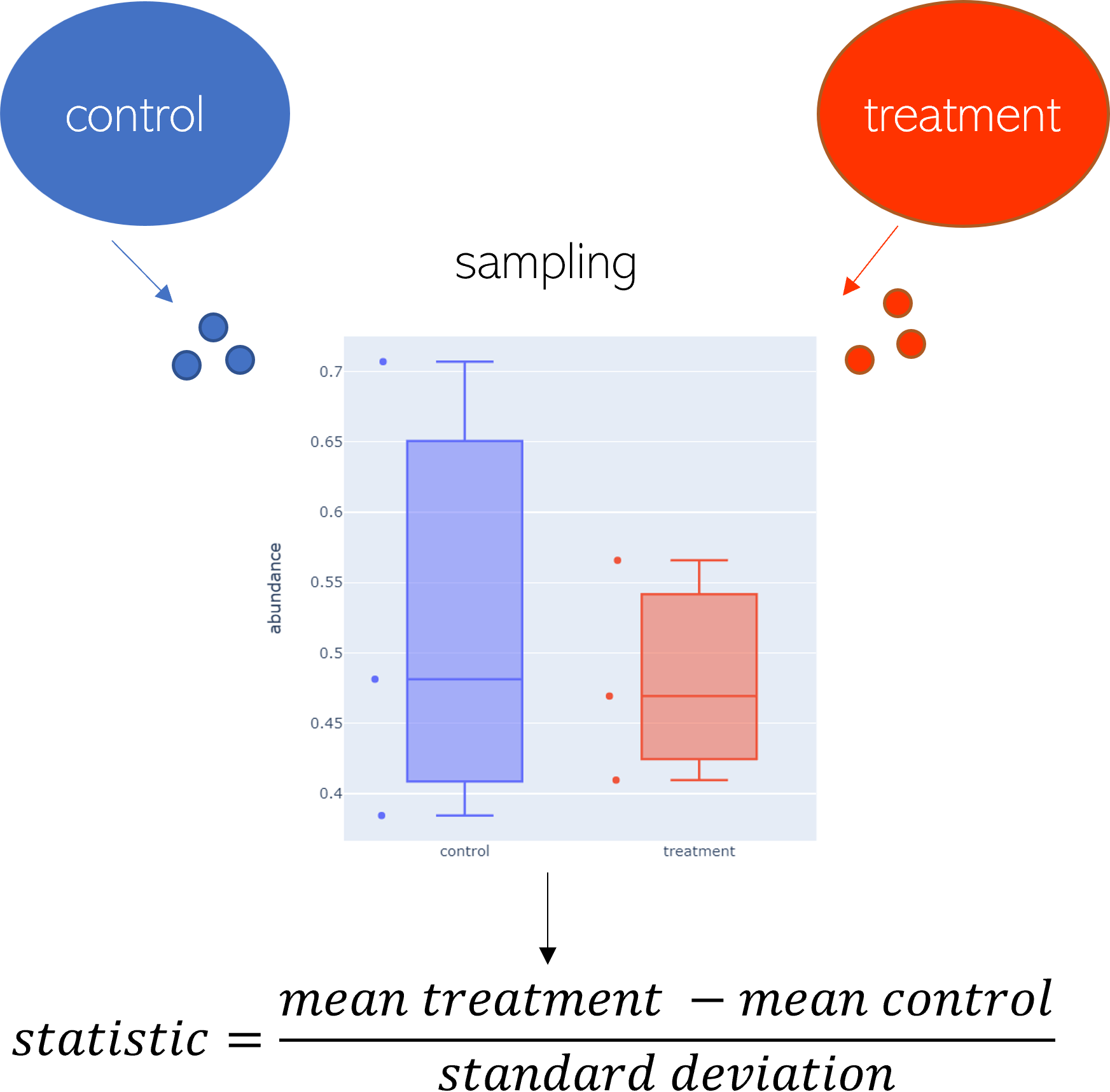
Figure 1: Sample workflow.
In figure 1 two samples, control and treatment, are compared. Each consists of three repeated measurements. The goal is to identify changes between the states. For that, the statistic is calculated.
Statistics
In this implemented version of SAM the t statistic is used.

This score of means relative to their standard deviation is sufficient to condense all replicate measurements into one score for each gene.
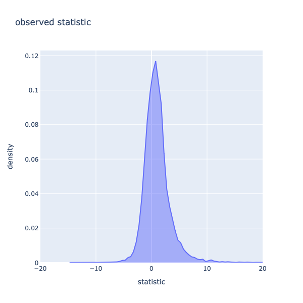
Figure 2: Histogram of statistics of the observed dataset.
When observing the histogram in figure 2, which shows the distribution of the statistics of the measured (observed) data from each gene, it is obvious that distribution is right-skewed. The shape of this histogram will be important later when comparing the observed data to the expected (permuted) data.
s0
Ideally, the variance of the statistic is only dependent on the statistic and not on the standard deviation (si). But that is not always the case.
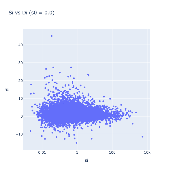
Figure 3: Statistics vs. their variance
In figure 3, the statistic (di) is plotted against the standard deviation (si). It can be seen that the variance of the statistics decreases with increasing sis (less spread on the Y-Axis). Including s0, an artificial fudge factor , aims to homogenize the variance of di in respect to si. The statistics di are calculated by dividing the mean through the pooled standard deviation, and therefore adding a constant to variance si leads to a decrease in the statistic.

Values with small standard deviations get affected stronger than the ones with higher standard deviations, ideally eliminating the relation between the variance of statistics and si. It is chosen as a percentile of si that minimizes the coefficient of variation of di.
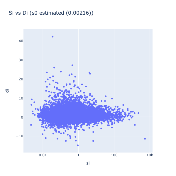
Figure 4: Statistics vs. their variance with s0 included.
Benefit of including s0 in the calculation of statistic scores is dampening the effect of large score values that result from near-zero gene expression. If a standard deviation is nearly zero, as in very reproducible measurements in replicates, it can lead to a strong t statistics overestimation. Both problems can be solved by the addition of s0 to the estimated standard deviation, because the denominator can not be smaller than s0, and therefore no infinite large scores can be produced.
Permuted data
For statistical comparisons, it is always important to have a reference, for example how the dataset would look like if there was a treatment, but no gene expression changed. This cannot be derived from the experiments. Tests that sample their own null distribution out of the given data, are often found in statistics and are coined permutation test. The advantage of using SAM for differential gene expression analysis is that the null distribution (treatment but no changes) is created directly from the observed data to estimate the behavior with no changes present (control vs. treatment). In the default version, the data are permuted by a column-wise Fisher Yates shuffle. To gain the expected statistics for SAM, a few steps have to be performed. First, the observed data are permuted (here 100 times) and ranked by their statistic. Afterwards, the mean statistic of all permutations of each gene is calculated (meaning: 100 datasets with all genes, condensed into one average dataset). This statistics can be plotted again in a histogram (see figure 3) and then compared to the observed statistics.
Calculating statistics for the permuted data allows to use it as a null distribution for comparison, because no links between prior scores and treatments are left.
The permutation, being a bootstrap method, leads to a random scrambling of the labels and each configuration is equally likely.
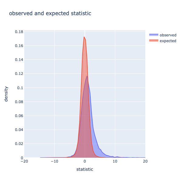
Figure 5: Histogram of statistics of expected and observed datasets.
In figure 5 are the histograms of observed and expected data displayed (comparison to figure 2). As previously described, the distribution of the observed data is right-skewed. The expected scores, in contrast, are more centered. The mode of the distributions with a bin-width of 0.5 is 0.11 for the observed data and 0.17 for the expected data. As mentioned previously, higher statistics indicate a higher possibility of real changes, and therefore differential gene expression can be expected. To investigate this further, the observed statistics are compared to the expected statistics.
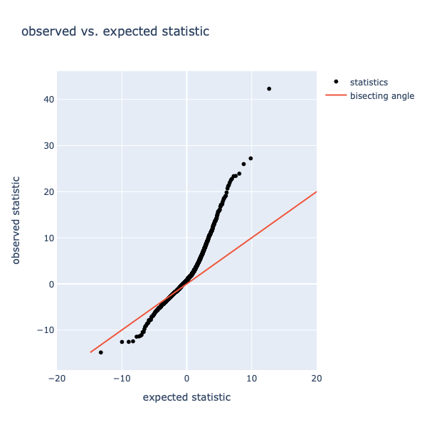
Figure 6: observed vs. expected statistics. The red line indicates the bisecting angle, the black dots represent statistics.
The bisecting angle is an indication where genes should be located if there is no difference between observed and expected scores. Datapoints deviating from the bisecting angle are potentially significantly different. The variation in the x-axis indicates the magnitude of the change, as more extreme values are more likely to be significantly different.
Significance
In order to determine significant changes an absolute distance from the bisecting angle (delta) is used as cutoff value. The cutoffs are obtained by selecting an arbitrary delta and finding the first gene and its corresponding statistic that exceeds the difference. This is done for the positive and negative direction to obtain the lower and upper cuts. The lower and upper cuts indicate the observed score where the absolute difference is the first time greater than delta. Every gene beyond that first exceeding threshold gene is called significant. To ensure that the differences are always increasing (or decreasing for the lower cut), a monotonizing function is applied. With that delta, the same step is performed on the expected datasets, where ideally no genes should be significant. The genes outside of the previously determined cuts are counted, and declared as false positive. With the information on how many genes are significant by chance (false positives), it is possible to calculate the False Discovery Rate by dividing the false positives through the amount of significant genes.
Figure 7: SAM results with FDR of 5%. The black line indicates the bisecting angle, the purple dashed line next to it the delta threshold. Lower and upper cuts are marked by grey dashed lines. Points colored red indicate genes that are downregulated, green indicates upregulation.
By varying delta, and therefore the difference between the statistics and the bisecting angle, it is possible to find more or less significant genes.
By increasing delta, the FDR decreases, and statistics have to be more extreme in comparison to the expected data to be called significant.
To clarify the meaning of the delta, a comparison with an FDR of 10% will be shown.
Figure 8: SAM results with FDR of 10 %. The black line indicates the bisecting angle, the purple dashed line next to it the delta threshold. Lower and upper cuts are marked by grey dashed lines. Points colored red indicate genes that are downregulated, green indicates upregulation.
Table 1: SAM Results with different FDRs.
| FDR 5% | FDR 10% | |
|---|---|---|
| s0 | 0.0021 | 0.0021 |
| pi0 | 0.63 | 0.63 |
| delta | 1.60 | 1.18 |
| upper cut | 2.65 | 1.88 |
| lower cut | -6.89 | -5.87 |
| positive significant | 2481 | 3969 |
| negative significant | 26 | 37 |
| non significant | 12338 | 10839 |
| significant called genes | 2507 | 4006 |
| median false positives | 125 | 400 |
Comparing the results with an FDR of 5% and 10%, it shows that s0 and pi0 remain unchanged because they are dependent on the dataset, not the FDR. In contrast to the results with an FDR of 5%, the delta of FDR 10% is smaller (1.6 vs 1.18) and therefore the cuts are also smaller. With an increasing FDR there is more uncertainty involved in the results, which can be seen at the greater number of significantly differentially expressed genes (2507 vs. 4006) as well as the higher number of false positives (125 vs. 400).
Modules of SAM
SAM is implemented as a modular test, meaning it is possible to add or exchange specific functions. Figure 9 is an overview of all steps performed in SAM.

Figure 9: Workflow of SAM.
pi0
Pi0 is another coefficient to ensure that SAM does not overestimate the FDR. It is estimated as the proportion of non-differentially-expressed-genes [2], so true positive null hypothesis. Multiplying it with the median false positive count helps getting closer to the real null distribution. To calculate pi0 the 25% and 75% quantile of relative differences of all performed permutations must be estimated, and the scores between those quantiles must be counted. Afterwards, the count must be divided through half the number of samples.
Example: Two different cells are tested (14845 genes each, FDR 5%). Cell 1 has a strong stress response, 11136 genes are significantly different expressed. Cell 2, in contrast, has a moderate response and only 2507 are significantly different expressed. The percentage of truly unchanged genes differs and the estimation of the null distribution relies only on the observed data. To account for this when calculating the median FDR, pi0 is included.
Delta
The variable delta is the absolute difference between observed and expected statistic, and it is calculated for each gene. With using delta as distance, cutoffs in the statistics can be determined and those correspond to an FDR.
Cuts
Asymmetric cuts are implemented to this Version of SAM because they take the possibility into account that a change in gene expression is not necessarily symmetric. This can happen when more upregulation than downregulation is present, or vice versa, and is not uncommon in biological experiments. The cutoffs are obtained by selecting an arbitrary delta (difference between observed and expected data) and finding the first gene and its corresponding statistic score that exceeds the difference. This is done for the positive and negative direction to obtain the lower and upper cut. Every gene beyond that first exceeding threshold gene is called significant. To ensure that the differences are always increasing (or decreasing for the lower cut), a monotonizing function is applied.
FDR
To call a gene significant in SAM it must exceed a difference (delta) between observed and expected statistics. In this implemented version each absolute difference is calculated and used to determine the corresponding FDR. The FDR is determined by these steps:
- find cutoffs (here, asymmetric cutoffs). Every datapoint exceeding this cutoff is called significant.
- count genes that exceed cutoffs in the observed data (significant genes)
count genes that exceed cutoffs in the expected data (median False Positives over all permutations)

The global FDR gives an overview about the amount of false positive genes within the reported significant elements.
By calculating the absolute difference and FDR for each gene, in contrast to samR, it gives the opportunity to select the used desired FDR more precisely without the need to search for a delta that would result in the FDR.
Another feature of SAM is the so-called local FDR or q Value, which is a gene specific value that gives the exact FDR at which that gene is called significant [3].
Limitations:
The implemented default version can right now process two class unpaired data, while samR can process timecourse and paired data, as well as some other types.
The way of permuting data can be a limitation, and there may be more efficient or fitting ones for your experiment.
However, SAM is designed to be modular and implementing your adapted permutation or statistic calculation is not a problem.
The last limitation of SAM is the estimation of the null distribution.
Because it uses a bootstrap method and generates the distribution only from existing data, problems arise if a large percentage of the genes are differentially expressed.
This can lead to a false null distribution, which is problematic because all calculations are based on the null distribution.
Alternatives
An alternative to SAM would be to perform multiple two sample t-tests and correct the p values subsequently. With this method the multiple testing errors would be a problem, and correction (e.g. Bonferroni) would lead to the loss of true positive findings. When working with high throughput data it is beneficial to use more tailored methods instead of the basic t test. SAM is a modular blue print for permutation tests, that is not limited to microarray data, but with alternative permutation patterns and exchangeable statistic calculations can be applied to several data (e.g. RNASeq, proteomics, and many more).
References
[1] Tusher V, Tibshirani R, Significance analysis of microarrays applied to the ionizing radiation response , 2001 DOI:10.1073/pnas.091062498
[2] Zhang S, A comprehensive evaluation of SAM, the SAM R-package and a simple modification to improve its performance, 2007 DOI:10.1186/1471-2105-8-230
[3] Tusher V, Tibshirani R, SAM "Significance Analysis of Microarrays" Users guide and technical document, SAM Users guide
- Hemerik J, Goeman J J, False discovery proportion estimation by permutations: confidence for significance analysis of microarrays, 2017 DOI:10.1111/rssb.12238
- Storey J D, Tibshirani R, SAM Thresholding and False Discovery Rates for Detecting Differential Gene Expression in DNA Microarrays, 2003 DOI:10.1007/b97411
- Lin et al., An investigation on performance of Significance Analysis of Microarray (SAM) for the comparisons of several treatments with one control in the presence of small-variance genes, 2008 DOI:10.1002/bimj.200710467
- Larsson O, Wahlestedt C, Timmons J A, Considerations when using the significance analysis of microarrays (SAM) algorithm, 2005 DOI:10.1186/1471-2105-6-129

