NB01b Plant Systems Biology

Download Notebook

1. Plant Systems Biology
2. Modeling growth
3. Insert growth data and display as chart
4. Calculation of growth rate and doubling time for cell cultures
5. Fitting biological growth curves
   1. Theory
   2. Model selection
6. Calculate cell doubling time
7. Questions
8. References

Plant Systems Biology

The general paradigm of Systems Biology clearly applies to plants, as they represent complex biological systems. The functioning of a plant as a biological system is the result of a combination of multiple intertwined and dynamic interactions between its components. In addition, most plants are sessile systems that have to face fluctuating environmental conditions, including biotic and abiotic stresses (Ruffel et al. 2010). The process of a biological system responding to changes in environmental conditions is termed acclimation. These molecular physiological responses represent a complex dynamic adjustment of the interplay between genes, proteins and metabolites that allows the organism to acclimate to the changing environment. The ability to acclimate ensures the survival of all living organisms and is therefore fundamental for the understanding of biological systems. Detailed knowledge about how plants acclimate to a changing environment is crucial especially in times of global climate change, as plants are of great importance for our quality of life as a key source of food, shelter, fiber, medicine, and fuel (Minorsky 2003).

The prominent model plant Arabidopsis thaliana is well suited for Plant Systems Biology studies because sophisticated experimental tools and extensive data collections are readily available (Van Norman et al. 2009). However, the importance of a model organism is not only coined by the availability of molecular tools to manipulate the organism, but also by its agricultural and economic impact like in the cases of tobacco, rice, maize or barley (Pãcurar 2009). Also, microalgae are of special economic interest due to their potential as biofuel producers (Cagnon et al. 2013). Additionally, the use of organisms with lower biological complexity facilitates the feasibility of System Biology studies and is an important factor to consider for the choice of a suitable model organism in Systems Biology.

The eukaryotic green alga Chlamydomonas reinhardtii is particularly well suited for Plant Systems Biology approaches. This unicellular freshwater and soil-dwelling alga has a single, cup-shaped chloroplast with a photosynthetic apparatus that is similar to that of higher plants (Eberhard et al. 2008, Merchant et al. 2007). Hence, results gained on photosynthesis processes in Chlamydomonas are likely to be transferable to higher plants. The nuclear, mitochondrial, and chloroplast genomes have been sequenced and tools for manipulating them are available (Merchant et al. 2007). Chlamydomonas cells have a size of ~10 µm and grow under photo-, mixo-, and heterotrophic conditions with a generation time of ~5-8 h (Harris, 2008). Chlamydomonas can be maintained under controlled conditions and environmental changes can be applied homogeneously and rapidly to all cells in a liquid culture. In contrast to multicellular organisms there are no influences by tissue heterogeneity. Even the influence of different cell cycle stages may be ruled out by performing experiments with asynchronous cell cultures (Bruggeman and Westerhoff 2007, Harris 2001). Finally, gene families in Chlamydomonas have fewer members than those in higher plants thus facilitating the interpretation of results involving many genes/proteins (Merchant et al. 2007).

Modeling growth

In order to solve real world tasks more convenient, F# provides a huge collection of additional programming libraries. Anything that extends beyond the basics must be written by a user. If the chunk of code is useful to multiple different users, it's often put into a library to make it easily reusable. A library is a collection of related pieces of code that have been compiled and stored together in a single file and can than be used an included. The most important libraries in F# for bioinformatics are:

• BioFSharp: Open source bioinformatics and computational biology toolbox written in F#
• FSharp.Stats: F# project for statistical computing
• Plotly.NET: .NET interface for plotly.js written in F# 📈

The first real world use case of F# in Systems Biology is to model growth for a defined cell number to see possible overexpression effects. Biologists often utilize growth experiments to analyze basic properties of a given organism or cellular model. For a solid comparison of data obtained from different experiments and to investigate the specific effect of a given experimental set up, modeling the growth is needed after recording the data.

This notebook introduces the most classical way to model growth of Chlamydomonas reinhardtii or any other growth data using F#.

Now, let's get started by loading the required libraries first.

#r "nuget: FSharp.Stats, 0.4.3"
#r "nuget: Plotly.NET, 4.2.0"

#if IPYNB
#r "nuget: Plotly.NET.Interactive, 4.2.0"
#endif // IPYNB

open System
open Plotly.NET
open FSharp.Stats

Insert growth data and display as chart

A standard cell culture experiment with cell count measurements will result in data like the following. Multiple cell counts (y_Count), each related to a specific timepoint (x_Hours).

// Code-Block 1

let exmp_x_Hours = [|0.; 19.5; 25.5; 43.; 48.5; 67.75|]
let exmp_y_Count = [|1659000.; 4169000.; 6585400.; 16608400.; 17257800.; 18041000.|]

// Such data can easily be display with the following code block.
// Chart.Point takes a sequence of x-axis-points and a series of y-axis-points as input
let example_Chart_1 = 
    Chart.Point(exmp_x_Hours,exmp_y_Count)
    // some minor styling with title and axis-titles.
    |> Chart.withTitle "Growth curve of Chlamydomonas reinhardtii cell cultures"
    |> Chart.withYAxisStyle ("Number of cells")
    |> Chart.withXAxisStyle ("Time [hours]")

example_Chart_1

No value returned by any evaluator

Calculation of growth rate and doubling time for cell cultures

The standard growth of an in vitro cell culture is defined by three phases. The lag phase in which the cells still acclimate to the growth conditions, the exponential growth, also called log phase, during which cell growth is exponential due to the iterative proliferation of cells into two daughter cells, and the stationary phase in which the growth rate and the death rate are equal. The stationary phase is typically initiated due to limitations in growth conditions, e.g. depletion of essential nutrients or accumulation of toxic/inhibitory excretions/products. The doubling time (or generation time) defines a time interval in which the quantity of cells doubles.

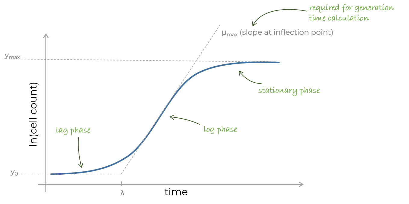
Figure 2: An exemplary growth curve.

Growth data always should be visualized in log space. Therefore the count data must be log transformed. When a log2 transform is applied, a doubling of the original counts is achieved, when the value increase 1 unit. Keeping that in mind, the slope of the growth function can be used to calculate the time it takes for the log transformed data to increase 1 unit.

The corresponding chart of the log transformed count data looks like this:

// Code-Block 2

// log transform the count data with a base of 2
let exmp_y_Count_Log = exmp_y_Count |> Array.map log2

let example_Chart_2 = 
    Chart.Point(exmp_x_Hours,exmp_y_Count_Log)
    |> Chart.withTitle "Growth curve of Chlamydomonas reinhardtii cell cultures"
    |> Chart.withYAxisStyle ("Number of cells [log2]")
    |> Chart.withXAxisStyle ("Time [hours]")

example_Chart_2

No value returned by any evaluator

After the log transform the exponential phase becomes linear. Since a y axis difference of 1 corresponds to a doubling of the cells the generation time can simply be estimated by determination of how many hours are required for the data to span one y axis unit. In this case it seems, that the time required to get from y=22 to y=23 takes approximately 10 hours.

As you may noticed we just determined the cell doubling time per eye. The formalization of this process is trivial.

• The y-value increment that is required for doubling can be calculated by log_x(2) where x defines the used base. So for log2 transformed data it is 1 (log2(2)).
• The generation time is calculated by dividing this y-value increment by the growth rate which is the steepest slope of the log transformed data (approximately 0.1 in the given data). The steepest slope in growth curves always occurs at the inflection point of the sigmoidal function shape.

So all we have to know is the performed log transform and the slope of the function at its steepest point and afterwards apply the following equation.

Equation 1: Calculation of the doubling time. Growth rate is the steepest slope of the log transformed count data.

For a log2 transform the numerator is 1.

Fitting biological growth curves

Theory

To derive the slope required for the doubling time calculation, the measured growth data points have to be modelled. In order to obtain a continuous function with known coefficients, a suitable model function is fitted onto the existing data. Many models exist, each one of them optimized for a specific task (Kaplan et al. 2018).

Linear model function example:

When a model function is fitted onto the data, there are endless possibilities to choose coefficients of the model function. In the case above there are two coefficients to be identified: The slope m and the y-intercept b. But how can the best fitting coefficients be determined?

Therefore a quality measure called Residual Sum of Squares (RSS) is used. It describes the discrepancy of the measured points and the corresponding estimation model. If the discrepancy is small, the RSS is small too.

In regression analysis the optimal set of coefficients (m and b) that minimizes the RSS is searched.

If there is no straightforward way to identify the RSS-minimizing coefficient set, then the problem is part of nonlinear regression. Here, initial coefficients are guessed and the RSS is calculated. Thereafter, the coefficients are modified in tiny steps. If the RSS decreases, the direction of the coefficient change seems to be correct. By iteratively changing coefficients , the optimal coefficient set is determined when no further change leads to an decrease in RSS. Algorithms, that perform such a 'gradient descent' methods to solve nonlinear regression tasks are called solver (e.g. Gauss-Newton algorithm or Levenberg–Marquardt algorithm). Introduction to RSS and optimization problems.

Model selection

Depending on the given problem, different models can be fitted to the data. Several growth models exist, each is specialized for a particular problem. See Types of growth curve or FSharp.Stats - Growth Curve for more information.

The selected model should match the theoretical (time) course of the studied signal, but under consideration of Occams razor principle. It states, that a approriate model with a low number of coefficients should be preferred over a model with many coefficients, since the excessive use of coefficients leads to overfitting.

An often used growth curve model is the four parameter Gompertz model.

The function has the form: Gibson et al. 1988.

where:

• A = curve minimum
• B = relative growth rate (not to be confused with absolute)
• C = curve maximum - curve minimum (y range)
• M = x position of inflection point
• t = time point

In the following, we will go through the necessary steps to calculate the generation time with the help of a Gompertz model. While the curve minimum and maximum are easy to define by eye, to estimate the remaining coefficients is a nontrivial task.

FSharp.Stats provides a function, that estimates the model coefficients from the data and a guess of the expected generation time. For Chlamydomonas the initial guess would be 8 hours.

// Code-Block 3

// open module in FSharp.Stats to perform nonlinear regression
open FSharp.Stats.Fitting.NonLinearRegression

// The model we need already exists in FSharp.Stats and can be taken from the "Table" module.
let modelGompertz = Table.GrowthModels.gompertz

// The solver that iteratively optimizes the coefficients requires an initial guess of the coefficients.
// The following function was specifically designed to estimate gompertz model coefficients from the data
// You have to provide the time data, the log transformed count data, the expected generation time, and the used log transform
let solverOptions = Table.GrowthModels.getSolverOptionsGompertz exmp_x_Hours exmp_y_Count_Log 8. log2

// sequence of initial guess coefficients
solverOptions.InitialParamGuess

No value returned by any evaluator

The initial coefficient estimations match the expectations.

• A = 20.7
• B = 0.099
• C = 3.4
• M = 19.5

// Code-Block 4

// By solving the nonlinear fitting problem, the optimal model coefficients are determined. 
// The solver iteratively changes the coefficients until the model function fits the data best.
let gompertzParams =
    LevenbergMarquardt.estimatedParams // The Levenberg Marquardt is used as solver
        modelGompertz    // The gompertz model is used as growth model
        solverOptions    // The initial guess of the coefficients
        0.1              // Parameter required from the solver
        10.              // Parameter required from the solver
        exmp_x_Hours     // The time data
        exmp_y_Count_Log // The transformed count data

gompertzParams

No value returned by any evaluator

The model coefficients were determined to be:

• A = 20.66
• B = 0.107
• C = 3.52
• M = 19.63

They are pretty close to the initial estimations that were determined in Code-Block 3 With the coefficients at hand, the model function can be filled with coefficients and can be used to create a fit to the data.

// Code-Block 5

// Create fitting function from optimal coefficients
let fittingFunction = modelGompertz.GetFunctionValue gompertzParams

// Fit the optimized model function to all x values from 0 to 70 hours.
let fittedValuesGompertz =
    [0. .. 0.1 .. 70.]
    |> Seq.map (fun x -> x,fittingFunction x) 
    |> Chart.Line
    

// combine the raw data and the fit into one chart
let fittedChartGompertz = 
    [
        example_Chart_2      |> Chart.withTraceInfo "raw data"
        fittedValuesGompertz |> Chart.withTraceInfo "gompertz model"
    ]
    |> Chart.combine

fittedChartGompertz

No value returned by any evaluator

Calculate cell doubling time

To calculate the doubling time it is necessary to determine the growth rate (gr) for equation 1. As discussed above the growth rate is the maximal slope of the model function. It always occurs at the inflection point, which we know is at x=19.628. After calculating the first derivative of the model function, we would be able to calculate the growth rate as the slope at the inflection point. Luckily, there is a short cut when using the Gompertz model. It allows the determination of generation times from its parameters (see Gibson et al. 1988 for details).

// Code-Block 6

let getGenTimeFromGompertz (parameterVector: vector) (logTransform: float -> float) =
    logTransform 2. * Math.E / (parameterVector.[1] * parameterVector.[2])

let genTime = getGenTimeFromGompertz gompertzParams log2

let gt = sprintf "The generation time is %.2f hours." genTime

No value returned by any evaluator

Questions:

1. Why is it useful to use a log2 transform rather than a ln, log10, or any other log transform?
   Hint: Define your own exponentially growing cell counts with a generation time of 1 and transform them using different log transforms.

2. Why is it not sufficient to fit the (raw or transformed) data using the possibilities Excel offers?
   Hint: Which models are available and why are these not always appropriate?

3. Calculate the generation time of the following data. Compare the time points of maximal slope of the raw data and the transformed data by eye. Without the log transform you are blind for the actual point of maximal growth.

let rawX_hours = [|0. .. 12.|]
let rawY_count = [|2.;2.2;2.9;5.;9.5;19.;38.;65.;85.;90.;91.;91.;91.;|]

References

1. Ruffel, S., Krouk, G. & Coruzzi, G. M. A systems view of responses to nutritional cues in Arabidopsis: toward a paradigm shift for predictive network modeling. Plant physiology 152, 445–452; 10.1104/pp.109.148502 (2010).
2. Minorsky, P. V. Achieving the in Silico Plant. Systems Biology and the Future of Plant Biological Research. Plant physiology 132, 404–409; 10.1104/pp.900076 (2003).
3. Van Norman, Jaimie M & Benfey, P. N. Arabidopsis thaliana as a model organism in systems biology. Wiley interdisciplinary reviews. Systems biology and medicine 1, 372–379; 10.1002/wsbm.25 (2009).
4. Pãcurar, D. I. Model organisms - a journey from the dawn of biological research to the post-genomic era. Romanian Society of Biological Sciences, 4087–4094 (2009).
5. Cagnon, C. et al. Development of a forward genetic screen to isolate oil mutants in the green microalga Chlamydomonas reinhardtii. Biotechnology for biofuels 6, 178; 10.1186/1754-6834-6-178 (2013).
6. Eberhard, S., Finazzi, G. & Wollman, F.-A. The dynamics of photosynthesis. Annual review of genetics 42, 463–515; 10.1146/annurev.genet.42.110807.091452 (2008).
7. Merchant, S. S. et al. The Chlamydomonas genome reveals the evolution of key animal and plant functions. Science (New York, N.Y.) 318, 245–250; 10.1126/science.1143609 (2007).
8. Harris, E. H. The chlamydomonas sourcebook. 2nd ed. (Academic, London, 2008).
9. Bruggeman, F. J. & Westerhoff, H. V. The nature of systems biology. Trends in microbiology 15, 45–50; 10.1016/j.tim.2006.11.003 (2007).
10. Harris, E. H. CHLAMYDOMONAS AS A MODEL ORGANISM. Annual review of plant physiology and plant molecular biology 52, 363–406; 10.1146/annurev.arplant.52.1.363 (2001).
11. Kaplan, S. et al. Comparison of growth curves using non-linear regression function in Japanese squail. Journal of Applied Animal Research 46, 112-117; 10.1080/09712119.2016.1268965 (2018).
12. Gibson, A., Bratchell, N., Roberts, T.A., Predicting microbial growth: growth responses of salmonellae in a laboratory medium as affected by pH, sodium chloride and storage temperature, International Journal of Food Microbiology, Volume 6, Issue 2, https://doi.org/10.1016/0168-1605(88)90051-7 (1988).